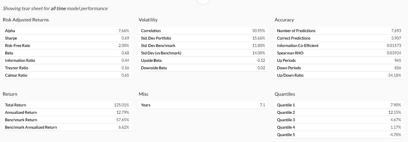
The tear sheet contains key performance metrics of the model over the selected graph range.
Accuracy and Quantiles metrics are based on raw model stock ranking output and will not change based on changes to portfolio settings. To improve accuracy a new model would need to be created and trained.
Returns and Volatility metrics are based on overall portfolio performance and will change if portfolio settings are modified. (See more on portfolio settings)
Risk Adjusted Returns Breakdown
| Description | |
| Annualized alpha | Alpha = Annualized Return – Risk-Free Rate - (Beta * (Benchmark Annualized Return - Risk Free Rate)). Alpha is a measure of the active return on an investment, the performance of that investment compared with a suitable market index. An alpha of 1% means the investment's return on investment over a selected period of time was 1% better than the market during that same period; a negative alpha means the investment underperformed the market. |
| Sharpe | Sharpe = (Annual Return – Risk-Free Rate) / Std. Dev of Portfolio The Sharpe ratio measures the performance of an investment (e.g., a security or portfolio) compared to a risk-free asset, after adjusting for its risk. |
| Risk-free rate | Risk-Free Rate = 0.5 The risk-free interest rate is the rate of return of a hypothetical investment with scheduled payment(s) over a fixed period of time that is assumed to meet all payment obligations. |
| Beta | Beta = Correlation * (Std. Dev of Portfolio / Std. Dev of Benchmark) Beta is a measure of the risk arising from exposure to general market movements as opposed to idiosyncratic factors. |
| Information ratio | Information Ratio = (Annualized Return – Benchmark Ann. Return) / (Std. Dev of (Portfolio Returns – Benchmark Returns)) The information ratio measures and compares the active return of an investment (e.g., a security or portfolio) compared to a benchmark index relative to the volatility of the active return (also known as active risk or benchmark tracking risk). It represents the additional amount of return that an investor receives per unit of increase in risk. |
| Treynor ratio | Treynor Ratio = (Annualized Returns – Risk-Free Rate) / Beta The Treynor ratio is a measurement of the returns earned in excess of that which could have been earned on an investment that has no diversifiable risk (e.g., Treasury bills or a completely diversified portfolio), per unit of market risk assumed. |
| Calmar ratio | Calmar Ratio = (Annualized Returns / the Absolute Value of the Largest Drawdown) The Calmar ratio is a function of the fund's average compounded annual rate of return versus its maximum drawdown. The higher the Calmar ratio, the better it performed on a risk-adjusted basis during the given time frame, which is mostly commonly set at 36 months. |
Return Breakdown
| Description | |
| Total return | Total Return = (Portfolio Value on End Date – Portfolio Value on Start Date) / Portfolio Value on Start Date The total return on a portfolio of investments takes into account not only the capital appreciation on the portfolio, but also the income received on the portfolio. The income typically consists of interest, dividends, and securities lending fees. |
| Annualized return | Annualized Return = (1 + Total Return) ^ (1 / Years) – 1 Annualized return is the total return calculated on an annualized basis in order to compare returns that may span over different time periods. |
| Avg. actual dividend yield | Avg. Actual Dividend Yield = The Actual Observed Dividend Yield of the Portfolio The dividend yield is the dividend per share, divided by the price per share. For the actual dividend yield, we are tracking the actual dividends received, so the yield will be 0 on day 1, rising to the actual yield by the end of year 1. |
| Avg. implied dividend yield | Avg. Implied Dividend Yield = The Implied Dividend Yield Based on the Weighted Historic Dividend Yield of All Stocks in the Portfolio The avg. implied dividend yield implies what the dividend yield is likely to be by calculating the weighted historic dividend yield for all stocks in the portfolio. |
| Benchmark return | Benchmark Return = (Benchmark Price on End Date – Benchmark Price on Start Date) / Benchmark Price on Start Date Benchmark return is the total return of the benchmark. It takes into account not only the capital appreciation on the portfolio, but also the income received on the portfolio. The income typically consists of interest, dividends, and securities lending fees. |
| Benchmark annualized return | Benchmark Annualized Return = (1 + Benchmark Return) ^ (1 / Years) – 1 Benchmark annualized return is the benchmark return expressed on an annualized basis. |
| Avg. benchmark dividend yield | Benchmark Dividend Yield = The Avg. Actual Dividend Yield of the Benchmark The dividend yield of the benchmark is the avg. actual dividend yield of the benchmark. For the actual dividend yield, we are tracking the actual dividends received, so the yield will be 0 on day 1, rising to the actual yield by the end of year 1. |
Volatility Breakdown
| Description | |
| Correlation | Correlation = Correlation of Period Returns by Day and Benchmark Returns by Day Correlation measures the relationship between the changes of two or more financial variables over time. For example, the prices of equity stocks and fixed interest bonds often move in opposite directions: when investors sell stocks, they often use the proceeds to buy bonds and vice versa. In this case, stock and bond prices are negatively correlated. |
| Std. dev portfolio | Std. Dev Portfolio = Standard Deviation of Period Returns by Day * SQRT (252) The standard deviation of the portfolio is a statistic that measures the dispersion of the portfolio returns relative to its mean and is calculated as the square root of the variance. It is calculated as the square root of variance by determining the variation between each data point relative to the mean. If the data points are further from the mean, there is a higher deviation within the data set; thus, the more spread out the data, the higher the standard deviation. |
| Std. dev benchmark | Std. Dev Benchmark = Standard Deviation of Benchmark Returns by Day * SQRT (252) The standard deviation of the benchmark is a statistic that measures the dispersion of the benchmark relative to its mean and is calculated as the square root of the variance. It is calculated as the square root of variance by determining the variation between each data point relative to the mean. If the data points are further from the mean, there is a higher deviation within the data set; thus, the more spread out the data, the higher the standard deviation. |
| Std. dev (vs benchmark) | Std. Dev (vs Benchmark) = Std. Dev of Portfolio Returns – Benchmark Returns The standard deviation vs. the benchmark, also known as tracking error, is a measure of the risk in an investment portfolio that is due to active management decisions made by the portfolio manager; it indicates how closely a portfolio follows the index to which it is benchmarked. |
| Upside beta | Upside Beta = Only Calculate Beta on Up Days Upside beta is the element of traditional beta that investors do not typically associate with the true meaning of risk. It is defined to be the scaled amount by which an asset tends to move compared to a benchmark, calculated only on days when the benchmark’s return is positive. |
| Downside beta | Downside Beta = Only Calculate Beta on Down Days Downside beta is the element of beta that investors associate with risk in the sense of the uncertain potential for loss. It is defined to be the scaled amount by which an asset tends to move compared to a benchmark, calculated only on days when the benchmark’s return is negative. |
Misc. Breakdown
| Description | |
| Total turnover | Total turnover is the amount of turnover relative to the equity in the portfolio, measured as buying. With $100 of equity, if you buy $100 of securities and sell $100 of securities you will have 100% turnover. |
| Annual turnover | Annual turnover is total turnover divided by the number of years the model is active. |
| Years | Years = (End Date of the model - Start Date of the Model) in days / 365 Years is simply the number of years the portfolio spans. |
Accuracy Breakdown
| Description | |
| Number of predictions | Number of Predictions = Total Number of Trades The number of predictions is simply the number of trades that the machine recommended over the period. |
| Correct predictions | Correct Predictions = Number of Trades with a Positive Return Correct predictions in the number of trades recommended resulting in a return that is greater than the benchmark. |
| Information co-efficient | Information Co-Efficient = 2 * (Correct Predictions / Number of Predictions) – 1 The information coefficient is a measure of the merit of a predicted value. In finance, the information coefficient is used as a performance metric for the predictive skill of a financial analyst. The information coefficient is similar to correlation in that it can be seen to measure the linear relationship between two random variables, e.g. predicted stock returns and the actualized returns. The information coefficient ranges from 0 to 1, with 0 denoting no linear relationship between predictions and actual values (poor forecasting skills) and 1 denoting a perfect linear relationship (good forecasting skills). |
| Spearman Rho |
Spearman RHO = The Correlation of the Rank Order of ML Value guidance: |
| Up periods | Up Periods = Number of Days with a Positive Return Up periods is simply a count of the number of days in the period with a positive return. |
| Down periods | Down Periods = Number of Days with a Negative Return Up periods is simply a count of the number of days in the period with a negative return. |
| Up/down ratio | Up/Down Ratio = Up Periods / (Up Periods + Down Periods) Up/down describes the percent of days that returns were positive versus total trading days. |
Return Quantiles Breakdown
| Description | |
| Return quantiles (Title) | The return quantiles are the top and bottom ranked stocks within this model. These do not change for new portfolios within the same model. Equities in Quantile 1 are ranked 5 stars, Quantile 2 are ranked 4 stars, and so on. Geometric Mean Return is primarily used for investments that are compounded. It is used to calculate average rate per period on investments that are compounded over multiple periods. We calculate it for each quantile. |
| Quantile 1 | Stocks ranked 5 stars. The stocks in this bucket are the ones our machine learning believes will perform best. Quantile 1 = (Geometric Daily Return of the First Quantile) ^ (252/1) -1 |
| Quantile 2 | Stocks ranked 4 stars. The stocks in this bucket are the ones our machine learning believes will perform better than average. Quantile 2 = (Geometric Daily Return of the Second Quantile) ^ (252/1) -1 |
| Quantile 3 | Stocks ranked 3 stars. The stocks in this bucket are the ones our machine learning believes will perform averagely. Quantile 3 = (Geometric Daily Return of the Third Quantile) ^ (252/1) -1 |
| Quantile 4 | Stocks ranked 2 stars. The stocks in this bucket are the ones our machine learning believes will perform below average. Quantile 4 = (Geometric Daily Return of the Fourth Quantile) ^ (252/1) -1 |
| Quantile 5 | Stocks ranked 1 star and below. The stocks in this bucket are the ones our machine learning believes will perform worst. Quantile 5 = (Geometric Daily Return of the Fifth Quantile) ^ (252/1) -1 |